Description
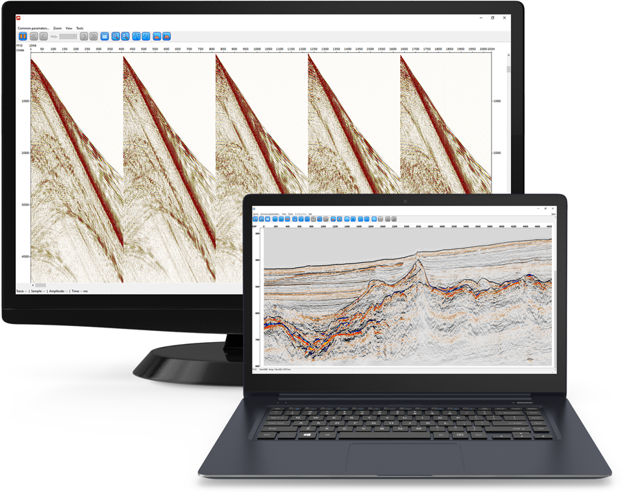
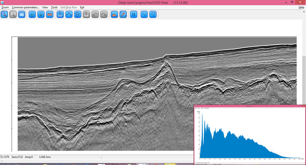
Marine High–Resolution Seismic Data Processing
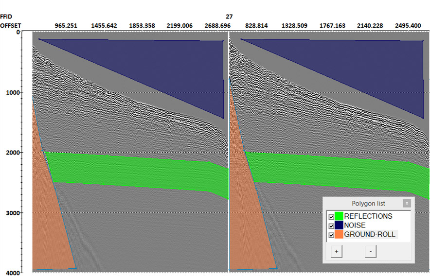
Advanced denoising, high–resolution offshore statics, designature (automatic wavelet estimation, deghosting, debubbling, deconvolutions), efficient demultiple algorythms for multi–channel (SRME) and even single–channel data (Zero–Offset Demultiple), 3D regularization, pre–stack and post–stack migrations—all these algorithms are available in RadExPro and are capable of improving the quality of the processing result significantly.
An experienced processor would particularly enjoy the outstanding flexibility of the software allowing even the most sophisticated processing scenarios to be easily implemented in the modern user–friendly interface—for only a fraction of the price of any big seismic processing system on the market.
Real–Time Marine Seismic Acquisition QC
What is marine real–time QC and why do I need it?
Real–time QC is dedicated for onboard seismic source and data quality control as soon as the data is received during marine seismic acquisition. It is aimed to identify any problems with seismic acquisition at the very same moment when they happen. This allows seismic crew to immediately fix the problems, minimizing related loss of operational time and money. Nowadays RT QC is the industry standard for marine seismic operations.
Typical real–time QC products are:
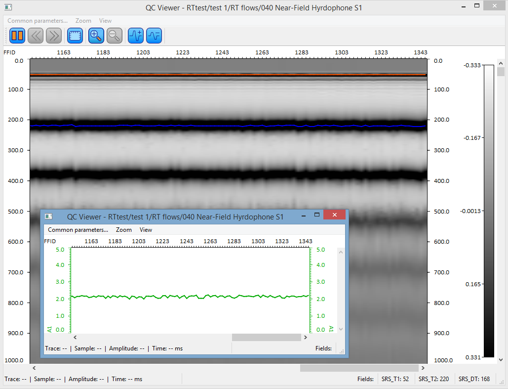
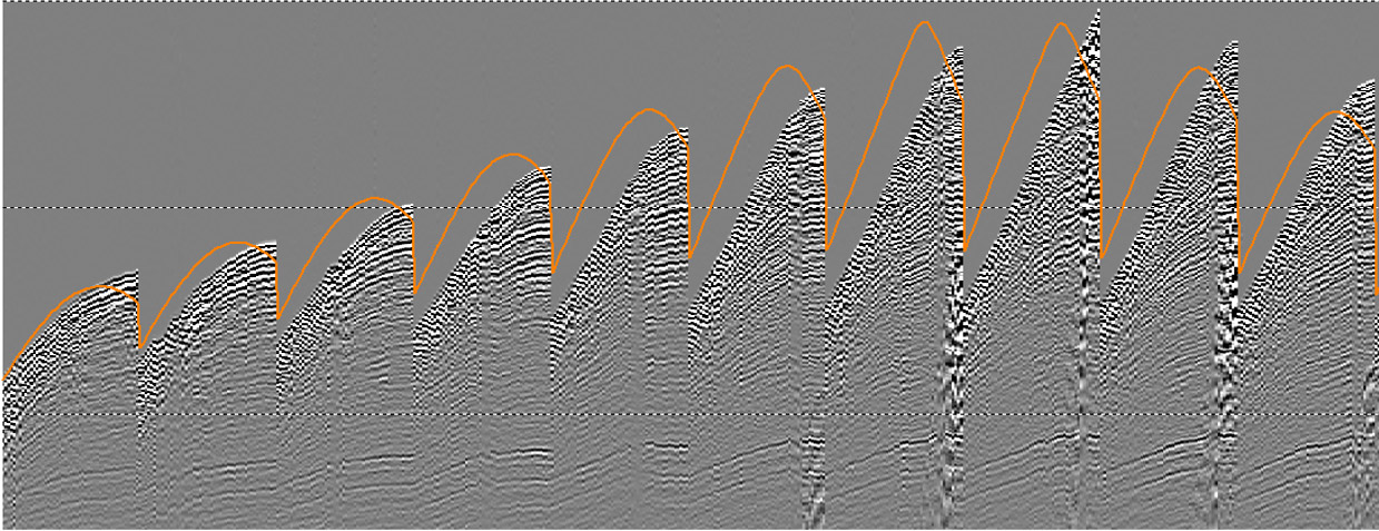
- Source control products: near–field hydrophone signature, bubble peak amplitude, bubble peak time, bubble time period, source towing depth, flip–flop source energy identity.
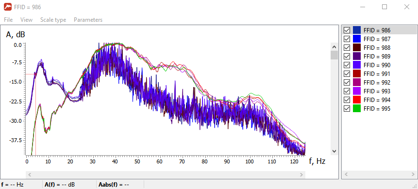
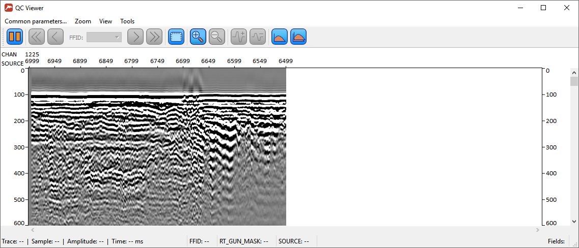
- Data control products: shot gathers, near–trace gathers, SOR/EOR/TARGET RMS amplitudes, signal/noise amplitudes, signal–to–noise ratio, real–time 2D stacks, frequency analysis.
This set of products controls most of the things happening on board, related to the seismic acquisition. By monitoring them, QC personnel and/or observers can easily identify “out of spec” issues like bad shots, bad or week channels, source air leakages, misfires, flip–flop source identity loss, low signal–to–noise ratio, strong noises, etc. Many of these issues requires immediate action and reporting.


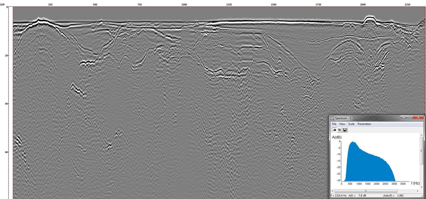
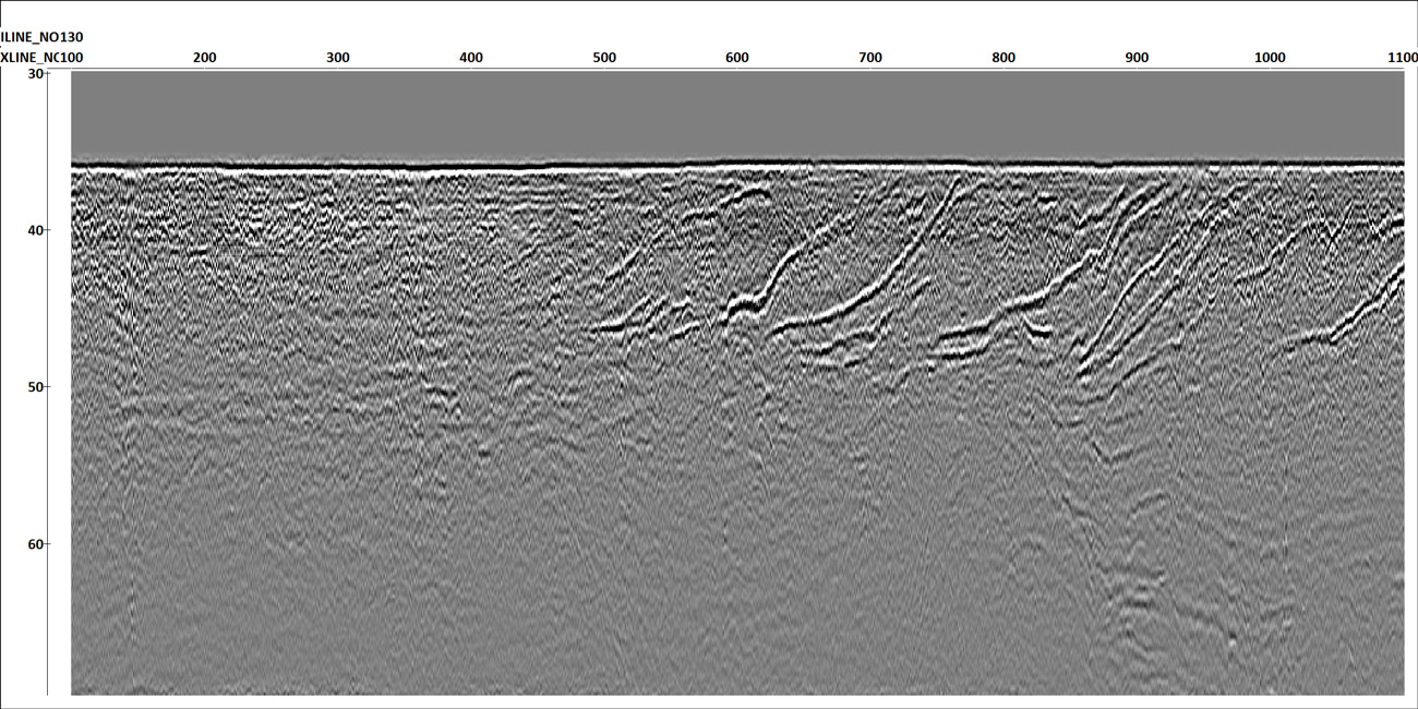
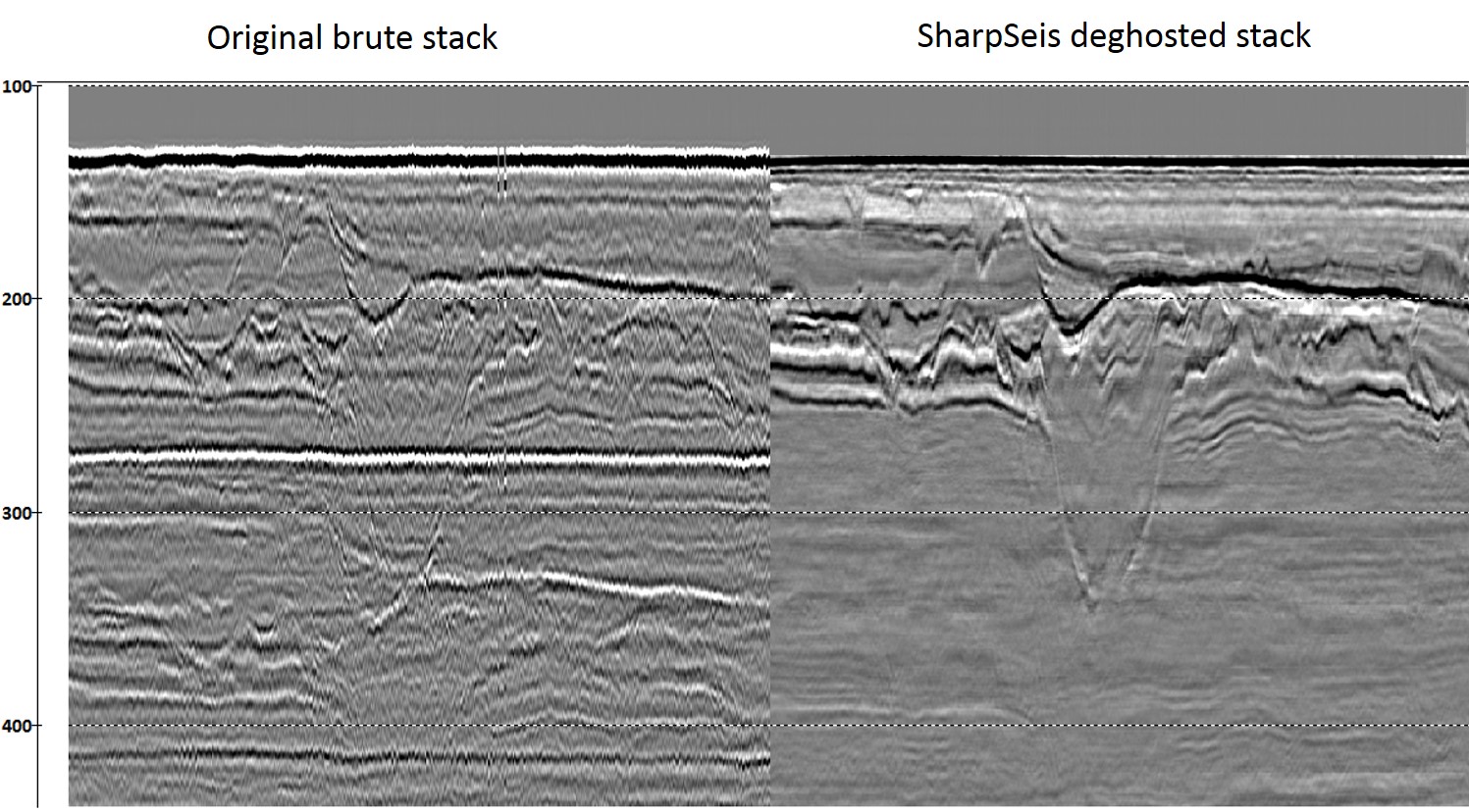
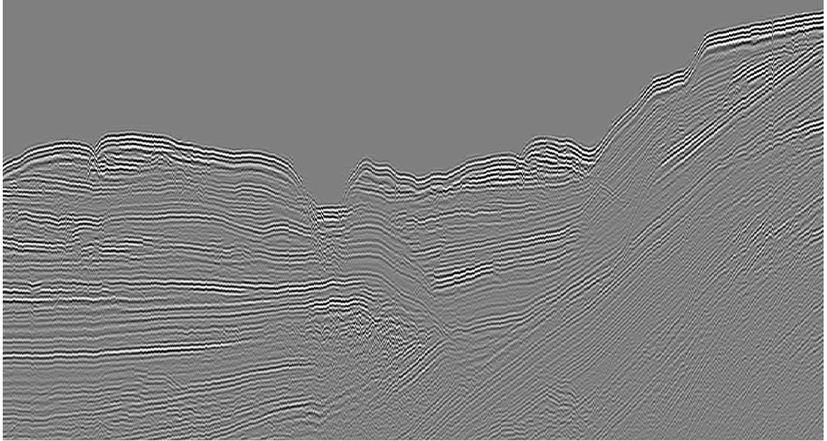
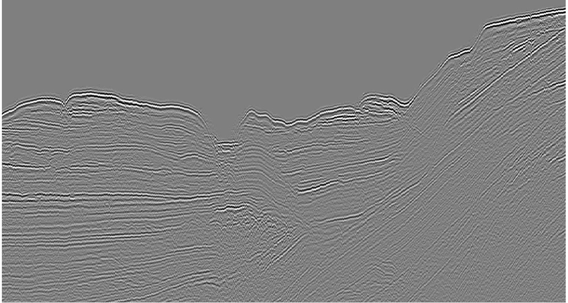
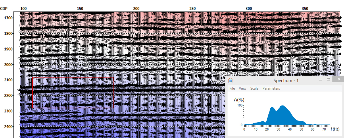
SharpSeis Deghosting/Broadband Processing
In typical marine seismic acquisition, a streamer towed on a given depth records not only an upgoing wavefield reflected from the subsurface, but also a downgoing field reflected from the sea surface and known as ghost wavefield. Destructive interference of the upgoing and the ghost wavefields creates a set of notch frequencies in the recorded spectrum, which results in limiting frequency band and decreasing resolution.
Algorithm specifications:
- Applicable for conventional marine seismic acquisitions—does not require specific acquisition solutions
- Efficient for different types of sources (airgun, sparker, boomer…)
- Applicable for both 2D and 3D data
- The algorithm is adaptive—can handle changing ghost time delays both in time and distance
The algorithm was presented at EAGE Near Surface Geoscience 2014—First Applied Shallow Marine Geophysics Conference byVakulenko et al (2014).
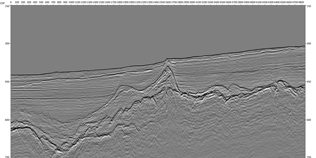
SharpSeis Deghosting helps one to recover a broader frequency spectrum, resulting in improved seismic resolution and image clarity.


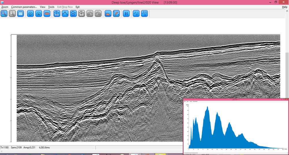
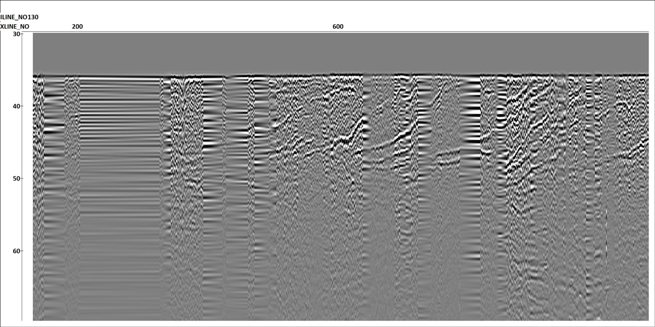
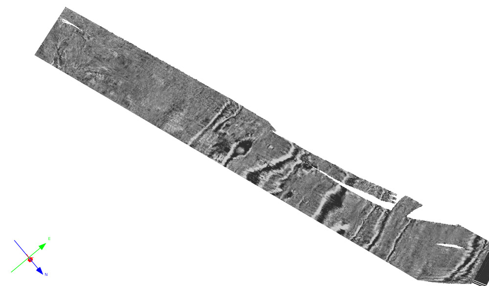
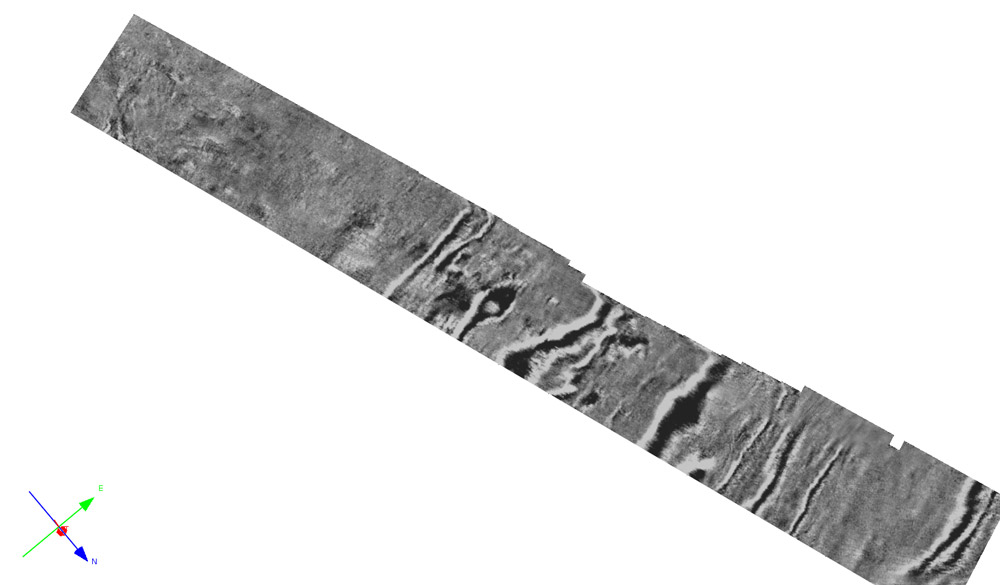
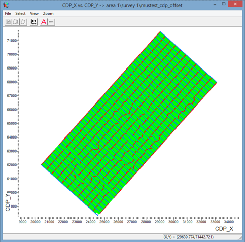
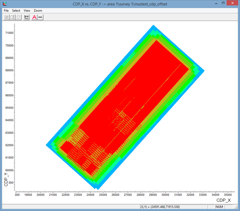
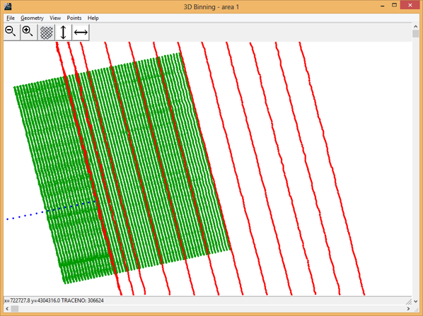
2D/3D Seismic QC and In–Field Processing
- Quick input of data of any size
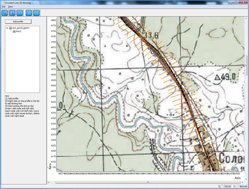
- Geometry assignment from SPS and P1–90 files
- Geometry QC using predicted times of direct wave arrival, as well as survey maps


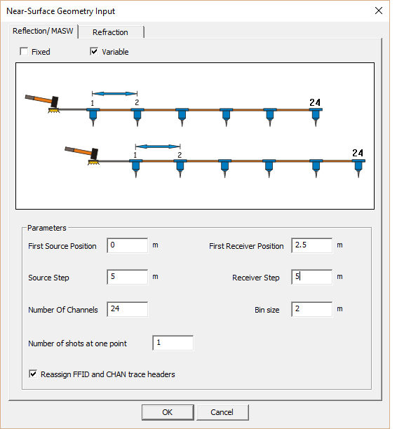
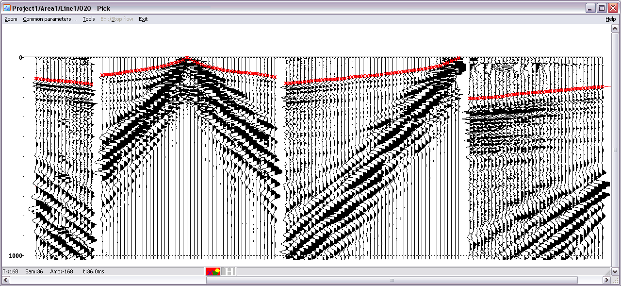
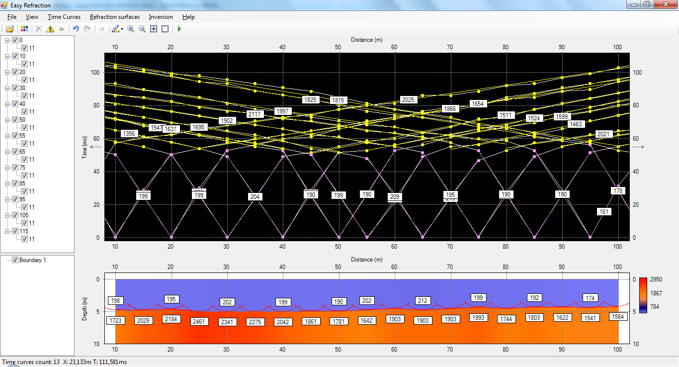
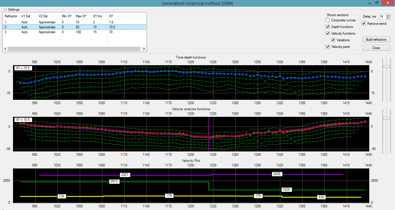
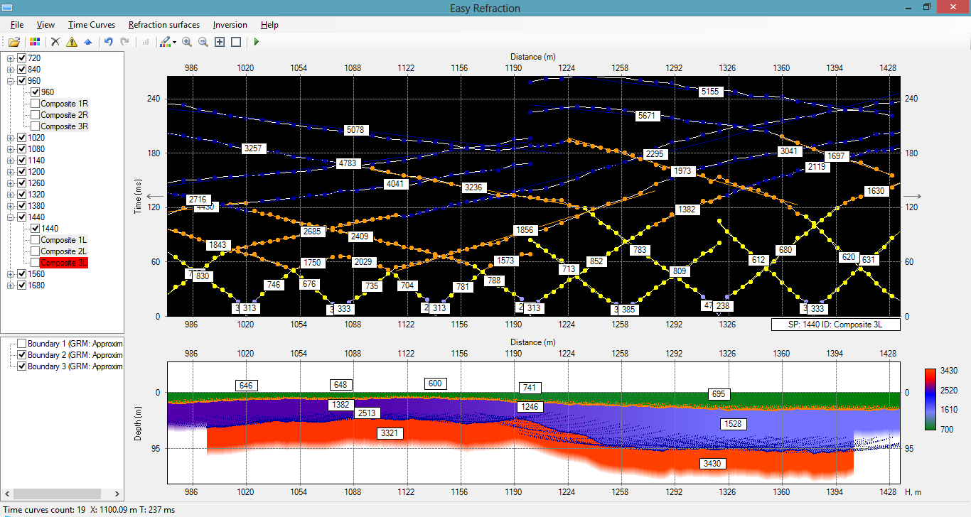
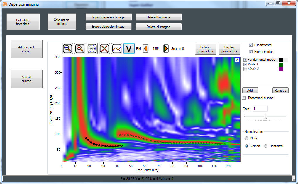
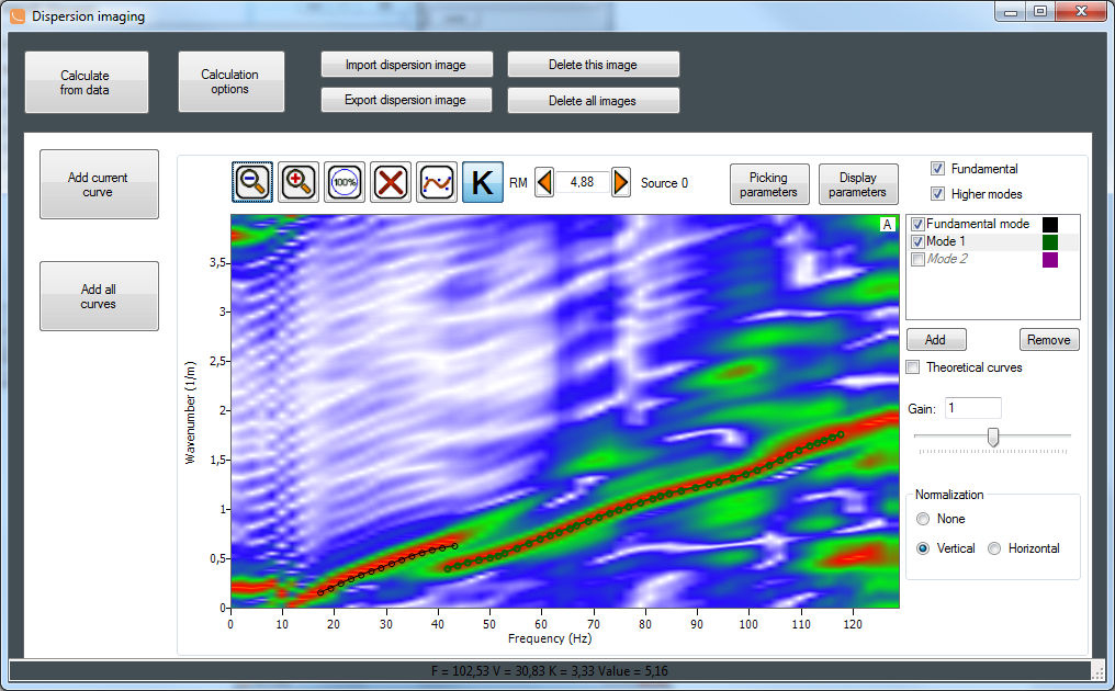
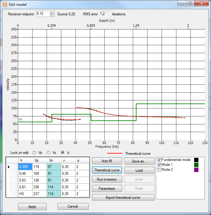
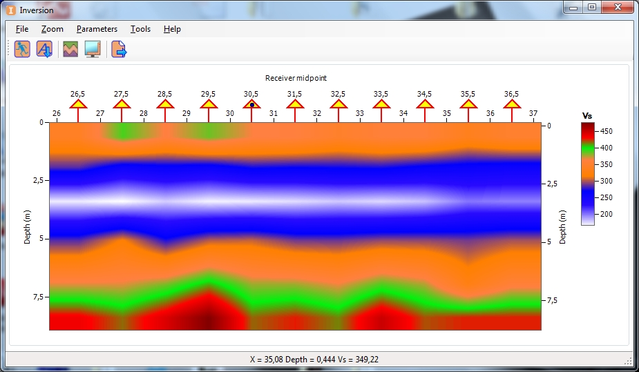
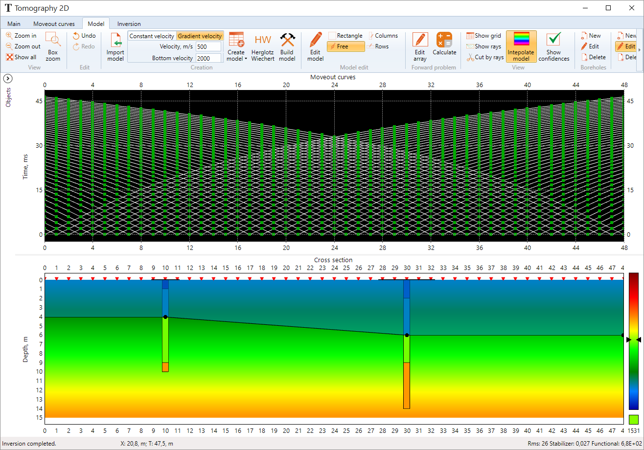
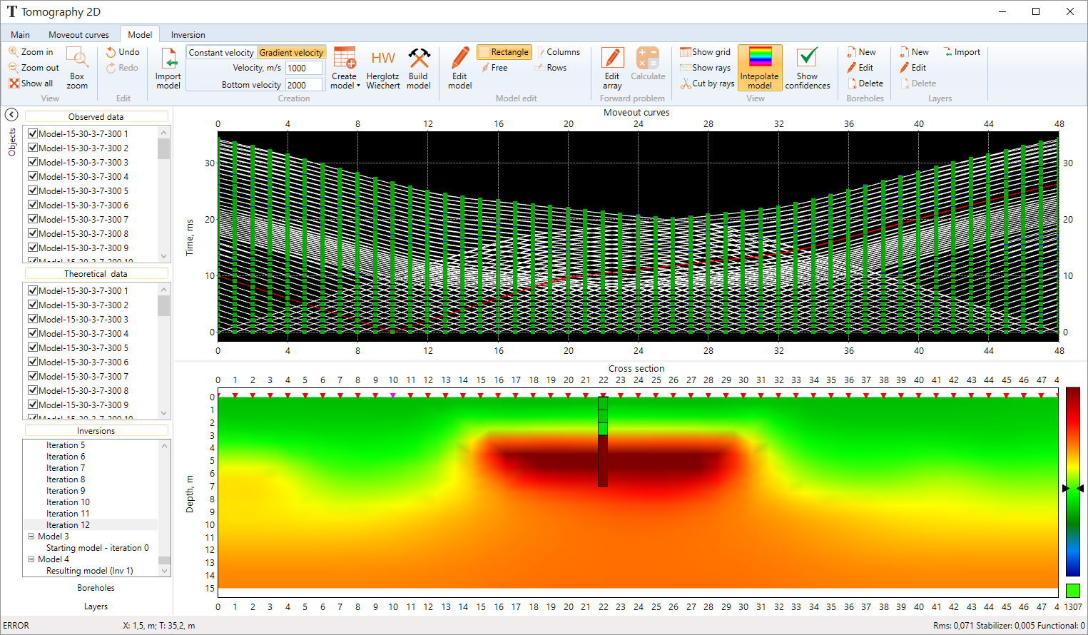
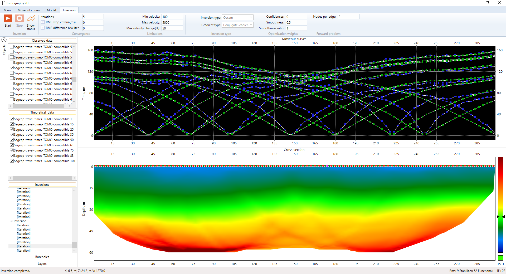
Near–Surface Data Processing
RadExPro provides a complete processing solution for all conventional near–surface seismic methods in one comprehensive package:
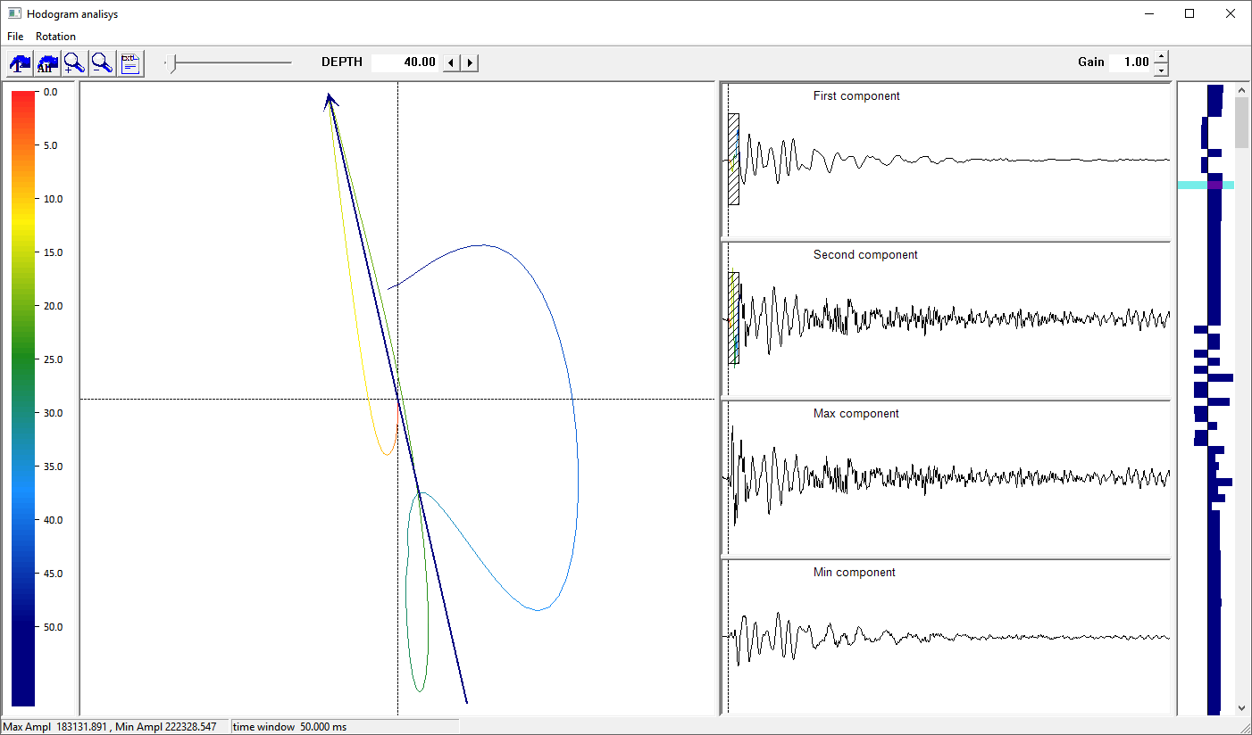
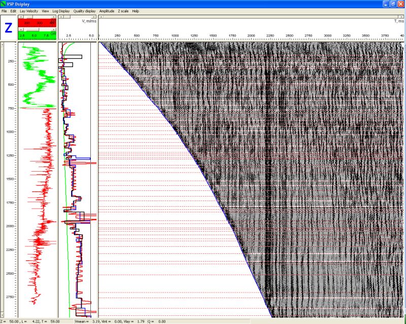
Vertical Seismic Profile
- Dedicated module for VSP survey geometry calculation and assignment, properly accounting for borehole deviations
- Efficient multi–component processing: hodogram analysis, 2C and 3C data rotation

Related products
-

AGTEK Earthwork 4D Suite 1.20 cracked
200 $ Add to cart Quick View -

Lantek Workshop (Manager, Wos, Capture)
150 $ Add to cart Quick View -
ReflectorCAD 1.5
150 $ Add to cart Quick View -

PointSense Total Package cracked version
200 $ Add to cart Quick View -

NAPA 2013 Ship Design Software
150 $ Add to cart Quick View -

Lantek Expert V33.03 (Cut, Punch, Quattro, Duct)
175 $ Add to cart Quick View -
VirtuSurv cracked version
130 $ Add to cart Quick View -

Intergraph CAESAR II v11 cracked version
120 $ Add to cart Quick View -
GPR-SLICE v7.0 cracked radar software
160 $ Add to cart Quick View -
Sale!

Intergraph CADWorx 2017 R1 cracked version
Original price was: 180 $.150 $Current price is: 150 $. Add to cart Quick View