DHI FEFLOW 10.0 full cracked release

Description

---

New 3D Supermesh Data Structure and more

In this new version, FEFLOW 10.0 comes with a new data structure for the 3D Supermesh, which follows a more geologically-oriented model description. The 3D Supermesh is aware of geological blocks and their connectivity to surfaces, as well as points and polylines add-ins within the blocks or crossing them. A new binary-fast file format (*.smh3d) is presented with major performance improvement. The new block concept replaces the old implementation using points (region markers) to keep track of the information during the meshing process.

Together with the new changes on the 3D Supermesh Data structure, FEFLOW comes with additional features related to the Supermesh such as a new workflow to build manually Supermeshes, multiple new tools and a new workflow to implicitly build geological models within FEFLOW (see more details below).

FEFLOW 10.0 brings a major review and improvement of Geode-FEFLOW tools such as Repair Surfaces and Re-triangulate Surfaces for explicit manipulation of 3D Supermesh objects. The Repair Surfaces algorithm offers now a fast decomposition of surfaces helping the user identifies properly the quality of the imported data into the 3D Supermesh, as well as the possibility to edit/delete unnecessary data.

Also, Repair Surfaces method is capable to identify the component relationships between blocks and surfaces. Geode’s mesh generator has been further extended to incorporate a new on-the-fly mesh optimization.

 3D Supermesh Structure with geological blocks.

More details about the 3D Supermesh and the new structure can be read in the section 3D Supermesh Design. Additional details about the explicit methods from Geode-FEFLOW tools can be read in the section 3D Supermesh Preprocessing.

Implicit Modelling of Geological Surfaces

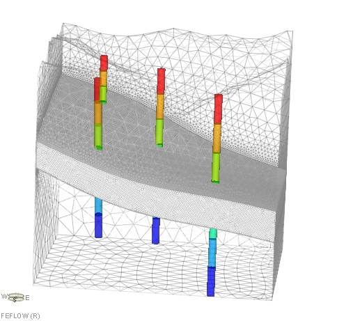
The 3D Supermesh format of FEFLOW 10.0 offers a new feature to include stratigraphic information in 3D models. With the new Implicit Modelling toolbar, we have now the possibility to perform implicit modelling of geological horizons (surfaces) from borehole (drill hole) data. This workflow allows you to build structural models directly in FEFLOW. The implementation of implicit modelling workflows in FEFLOW is a significant milestone to support many users further workflows with 3D unstructured meshes and help them to reduce the dependency on third-party geological software.

The workflow is illustrated in the Figure below: (left) the original 3D Supermesh with a set of boreholes and (right) the implicitly-generated surfaces perfectly matching the input boreholes.

 

Implicit modelling workflow: 3D Supermesh before (left) and after (right) the geological structure has been built.

Moreover, FEFLOW finite-element mesh built with Geode’s mesh generator allows the full control of the discretization level. The user can impose edge-size constraints for the tetrahedral mesh at the block level, at the implicitly-generated surfaces (contacts between blocks) and at any other geometrical add-ins (point, polylines and/or fault surfaces).

Final FEFLOW mesh generated with Geode-FEFLOW tools based on implicitly-generated surfaces.

Further details about the new workflows can be found in the section Implicit modelling.

Equation of State (EOS)

In deep geothermal systems, temperature may exceed 100°C,  but the boiling point depends on pressure, so a liquid phase is maintained as pressure increases with depth. Thus, no multiphase treatment is required; however, the density changes become nonlinear and viscosity changes become significant.

In order verify the validity of the single-phase flow, FEFLOW 10.0 introduces a new Auxiliary parameter named Temperature relative to boiling. Based on a pressure-dependent boiling point calculation, the parameter indicates the regions, where there may a potential change of phase.

New Auxiliary Parameter: Temperature relative to boiling.

The Equation of State (EOS) used through multiple numerical methods has been extended in FEFLOW 10.0. In a new page Equation of State under the Problem Settings dialog, you can now find all the options to control fluid density and fluid viscosity. Fluid density can be nonlinearly expressed as a function of Concentration, Temperature and Pressure. Fluid density and Fluid viscosity are now FEFLOW’s primary variables. Their values are directly computed at local finite element nodes, rather than indirectly via concentration or temperature, as it has been done in previous software versions. This new implementation provides more accuracy on the calculations. The new implementation of the EOS extends FEFLOW’s range of application, where temperature can range from 0 to 300°C, concentration from 0 to 300 g/l and fluid pressure up to 100 MPa (1000 bar).

Also, for cases, where the fluid density can have a linear dependency, the parameters Density ratio and Expansion Coefficient can be assigned globally or as per-element.

All reference parameters such as concentration, temperature, fluid density and fluid dynamic viscosity are accessible through the new EOS page.

New page Equation of State in the Problem Settings dialog.

More details about the new EOS page are documented in this section.

Extension of the Standard Transport Equation

Since the very beginning, FEFLOW has offered two transport formulations to be applied for Mass and Heat modelling cases. These are the so-called Convective Form of the Transport Equation (CFTE) and Divergence Form of the Transport Equation (DFTE). The new implementation considers a Standard Transport Equation using a total-flux definition for the transport boundary conditions. This new Standard Transport Equation is now the default version in FEFLOW 10.0 and onwards.

The Standard Transport Equation is based on the former Convective Form of the Transport Equation, but considering a total-flux formulation for the boundaries. In concrete, the Mass and Heat Boundary Conditions of 2nd, 3rd and 4th kind by default allows a total flux. When the boundary portion is impermeable to flow, flux naturally becomes purely dispersive / diffusive.

The budget calculations has been extended to incorporate as well these changes. The Standard Transport Equation reports the mass/heat budgets the way the DFTE does.

Legacy formulations are still available through Transport Settings page.

Reference projection and online visualization

FEFLOW 10.0 includes the awareness of real-world coordinate systems. The user can now define a reference projection to FEM and Supermesh projects. A reference system for the FEFLOW project must be always in projected coordinates. However, map files imported for visualization and other purposes could have a different coordinate system (e.g. geographic coordinates). With the help of a new on-th-fly re-projection feature, FEFLOW knows exactly where to locate the data.

The new Map Projection dialog under the menu Edit comes an extensive list of map projections helping you to define the right information to your FEFLOW’s projects. If imported map files already contains reference system (e.g. a Shapefile), with a simple right-click, you can ask FEFLOW to use the same projection for the FEM model or Supermesh.

In addition to these great functionalities, FEFLOW 10.0 has the possibility to include online background maps for your projects. You can invoke the new option Add Online Maps from the context menu of the Maps panel. Online background maps come with multiple visualization style giving the maximum flexibility for your projects.

Using Online Maps within the FEFLOW graphical interface: detail on how to include an online map (left) and zooming to a specific area to review project details (right).

Further information about these new features can be found in the sections Map Projections and Maps Panel.

Isofeatures as Spatial Entities

The visualization of modelling results (Process variables) such as Pressure, Hydraulic Head, Concentration and Temperature, as isosurfaces is a common operation for many FEFLOW users. Such as surfaces are rendered in the 3D View based on any user-defined iso-value.

In FEFLOW 10.0, any isosurface can be used now as canvas for visualization. In concrete, FEFLOW can plot anything (nodal or elemental quantities) on the 3D surface. A typical example is to use the Zero-Pressure Isosurface (water table) to plot Hydraulic Head or Concentration on the water level. The surfaces can be used as any other entities for visualization. Under the Spatial Entities panel, we have a new section named Isofeatures listing all available surfaces for visualisation.

In the example below, you can observe the visualization of Hydraulic-Head distributions plotted on the groundwater table (Zero-Pressure Isosurface). Due to the decrease of the groundwater table (due to mine dewatering), the isosurface consequently decreases over time. Every time the Isofeatures is rendered, then the Hydraulic-Head Fringes are updated accordingly.

Visualization of Hydraulic-head distribution plotted at the water table (zero-pressure isosurface). An example of open-pit dewatering.

Extended Budget-History Charting

A very popular FEFLOW’s feature is the recording on the budgets in charts. This operation is named Budget-History Charting. Traditionally, the activation of budget recording has been done through the context menu of specific nodal selections. As a complementary workflow, in the previous release, the definition of budget groups was made accessible via the Observation Data dialog.

FEFLOW 10.0 provides an extension of the Observation Data dialog. The budget groups, i.e. nodal selection used for Budget-History Charting, are enhanced with multiple recording modes. Budgets amount can be recorded based on inflow, outflow or net quantities. The “net” quantity option is the traditional. Such level of versatility helps you for further analysis of the modelling results without limits.

Activation of the “Out” recording mode for a given nodal selection.

Heat Period Budget chart presenting results in two recording modes (in and out). An example of a Aquifer Thermal Energy Storage.

You will find more information about this new functionality in the Budget-History Charting section.

New 1D hydrodynamical coupling

The former IfmMIKE11 is now officially replaced by FEFLOW piMIKE1D. In the previous release, a Beta version of the coupling was offered on demand. Today, we are officially launching new solution. FEFLOW piMIKE1D offers a native coupling between FEFLOW and MIKE 1D engines for integrated groundwater and surface water modelling, respectivaly. MIKE 1D is the new DHI’s generation of surface water engine and is the successor of the former MIKE 11. MIKE 1D engine is part of MIKE+ products.

FEFLOW piMIKE1D supports the coupling between an existing Node Selection and a River Network file from MIKE 1D. It is not required to previously define a Fluid Transfer BC on the target Node Selection, as it’s automatically set by the coupling.

For user previously working with the old coupling, FEFLOW piMIKE1D supports you to easily migrate to the new framework. MIKE 11 files (*.mhydro, *.sim11) can be read and automatically used for the coupling in FEFLOW.

Further details about the hydrodynamical coupling can be read in this section.

Visualization of Hydraulic-head distribution plotted at the water table (zero-pressure isosurface). An example of open-pit dewatering.

New FEFLOW-Python APIs

FEFLOW 10.0 extends the FEFLOW-Python Programming Interface by supporting the new 3D Supermesh Data Structure. All these methods APIs for the 3D Supermesh are accessible through the FEFLOW-Python’s module named PySMH. The new 3D Supermesh methods in Python allows to create entirely a 3D Supermesh project (*.smh3d) and edit/include additional geometries such as polylines, surfaces, multipoints, horizon points and blocks. In additional, all the Geode-FEFLOW methods such as Repair Surfaces, Re-triangulate Surfaces and Generate Implicit Surfaces are also accessible through the Python interface.

A new implementation is offered now to fully control the conductivity tensor through standard FEFLOW IFM Python.

Now you can control the map projections directly via Python with the methods doc.setGeoCoordinateSystem() and doc.getGeoCoordinateSystem().

Several usability improvements and others

Beside all major improvements presented above. FEFLOW 10.0 comes with several usability improvements. One example is the new option of “Handling” the visualization of parameters during the navigation. The visualization of certain parameters (such as Darcy velocity vectors, isosurfaces, etc.) in the 3D View may be computational expensive, especially for large models. FEFLOW has enhanced the performance by simply turning off the visualization during navigation and certain operations (zoom, rotation, translation, among others). After mouse release, all the parameters will be automatically displayed again in the view as usual.

FEFLOW 10.0 introduces a second verification of the Minimum Hydraulic-head constraint assigned to a Well BC. This second verification of the constraint avoids cases of unwanted infiltration. More details can be found in the section Boundary Condition Constraints.

Last but not least, the release comes with a major upgrade of the graphic programming interface (Qt) used in FEFLOW.  Also, software problems related to the stability and malfunctioning of certain operations have been corrected.